Today, you can use Dijkstra’s pathfinding algorithm to find the shortest path from the gate to cafeteria. After understanding what it is & how exactly it works, we’ll implement it using Python. Later, we’ll implement a more better variant of it called A* algorithm. But in this post, we’ll keep ourselves to Dijkstra algorithm. If you just need pseudocode or python implementation, scroll down.
In a nutshell
Dijkstra’s algorithm simply takes a graph in its input, travels through its edges, and tries to find the shortest possible distance from source point to destination point. We use it (or its variants) to find the shortest distance from enemy to player characters in video game, or we can use it in applications such as maps to find better route.
In nutshell, this algorithm starts at a source node & checks all unvisited nodes & their neighbors. Whenever it encounters a neighbor, it checks if the distance to it through this current node is more shorter than the previously known distance. If so, update new distance to shorter one, else keep searching until all nodes are eventually set to their most optimum distance from source. After this whole thing, we just usually extract our node of interest, which is destination node.
Understanding Dijkstra’s Algorithm
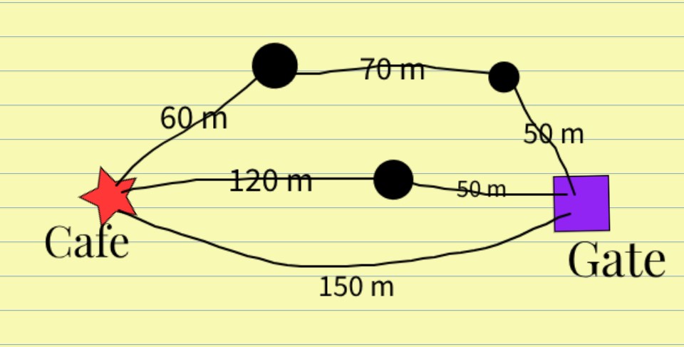
Looking at the above map, you can easily see that the 150 m path is the shortest, since other roads end up having more meters of distance. But how does Dijkstra’s algorithm figures this out is a bit different. First of all, we need to represent our map in the form of a graph data structure since this computer algorithm takes a graph in its input & returns the shortest path to the destination as its output.
A graph is a structure in which there are points connected through lines. We call points as nodes & lines connecting them as edges. Each edge can have different length. This is not necessarily “length” as it can be any kind of variable here. If you are making a graph of your city’s roads, you can assign the road’s condition & traffic as its weight so the more bigger the value of edge weight, the bad the road’s condition & the more difficult it will be to pass through it. So edge weight can represent any entity. Here we used distance as the edge’s weight (in meters).
In Dijkstra’s algorithm, one thing is very important: the algorithm explores all the paths for every node. So if a particular path that was visited first had a distance of, for example 10 & after a while, it discovered that while passing through a different path, it took distance of 8 to reach there, the algorithm will immediately update the distance to this node. And this happens every time the new smaller distance is found. The fact is, we are interested in the distance to a particular node only, so we simply ignore other distances & only use its value after algorithm has completed its operation.
The Algorithm’s Process:

- Initially, since it doesn’t know anything, it simply assigns the distance to our starting point (source node) to be equal to zero. And assigns infinity distance to all other nodes! It means that we do not know distances to any other nodes. Also, to keep track of all the visited & unvisited nodes, we need to initialize priority queues (or min-heap). The priority queue is used to store nodes along with their current calculated distances from the source node (at this time, these distance may not be optimal, since later another possible path to the same node can yield a better distance, until algorithm completes).
- After the stage has been set up in above step, the process begins by getting the node from the “`unvisited_nodes“` that is the neighbor of source node & has the smallest distance from it. The edge with smallest weight will be selected and node connected to it will be taken. We call this nearest-to-source node as “`currentNode“` since we will explore it further. Since we have picked it from “`unvisited_nodes“`, we will now remove it from the “`unvisited_nodes“` queue.
- Now, in a loop, we will look at each node connected with our currentNode. We call it neighbor. For every neighbor, we check if the distance assigned to it earlier was greater then currently found distance through this currentNode. If it was greater & this one is smaller, we will override the value of this neighbour’s distance to current value (as its smaller, more optimal) & we will also override the “previous_node” to be the current node (since, we will be returning this linked list of nodes as output, with each node connected to previous all the way from source to destination nodes; to keep track of the “path” itself).
- Process 2 above is a loop iterating over all the nodes from unvisited_nodes queue. And process 3 is the nested loop within currentNode’s loop & iterates over currentNode’s neighbors. After both process have completed, and program successfully exits the loops, we simply return both our path (that was a list) & the distances (to every node, in case we need it).
Confusion-solver notes
- Although Dijkstra’s algorithm looks at the shortest distance neighbour initially for lookup, it doesnt mean that it ignores the long-distance neighbours. Since later in the life of this algorithm, it may discover what initially seemed a longer distance was in fact a shorter one compared to the combined distances of the path it took initially thinking that to be efficient.
- Dijkstra’s algorithm takes a source, and as it traverses the graph, it sets the distance to EVERY other node that it travels in such a way that if its previous distance was longer & current one is shorter, it updates the value of distance & the pointer to previous node (to keep track of path). After the whole algorithm is completed, we pick the node from the graph that we call destination & use its previous node pointer to trace the path back to source vertex.
Pseudo-code
function Dijkstra(Graph, source)
     for each point in Graph.points:
         distance[point] ← INFINITY
         previous_point[point] ← UNDEFINED
         add point to Queue
     distance[source] ← 0

     while Queue is not empty:
          currentPoint ← point in Queue with minimum distance[currentPoint]
          remove currentPoint from Queue

          for each neighbor of currentPoint still in Queue:
              alt ← distance[currentPoint] + Graph.edges(currentPoint, neighbor)
              if alt < distance[neighbor]:
                  distance[neighbor] ← alt
                  previous_point[neighbor] ← currentPoint

      return distance[], previous_point[]
Python Implementation
import heapq

def dijkstra(graph, start):
    # Initialize distances and visited set
    distances = {vertex: float('infinity') for vertex in graph}
    distances[start] = 0
    visited = set()

    # Priority queue to keep track of the next vertex to visit
    priority_queue = [(0, start)]

    while priority_queue:
        # Get the vertex with the smallest distance
        current_distance, current_vertex = heapq.heappop(priority_queue)

        # Skip if the vertex has already been visited
        if current_vertex in visited:
            continue

        # Mark the vertex as visited
        visited.add(current_vertex)

        # Update distances for neighboring vertices
        for neighbor, weight in graph[current_vertex].items():
            distance = current_distance + weight

            # If a shorter path is found, update the distance
            if distance < distances[neighbor]:
                distances[neighbor] = distance
                heapq.heappush(priority_queue, (distance, neighbor))

    return distances

# Example usage
graph = {
    'A': {'B': 1, 'C': 4},
    'B': {'A': 1, 'C': 2, 'D': 5},
    'C': {'A': 4, 'B': 2, 'D': 1},
    'D': {'B': 5, 'C': 1}
}

start_vertex = 'A'
result = dijkstra(graph, start_vertex)

print(f"Shortest distances from {start_vertex}: {result}")